Executive Summary
Problem Summary
With the advent of smartphones and the consumer economy, there has been a revolution in the ways that people consume products and content. At the same time, digital music and digital music distribution platforms have become some of the most widely accessible and highly consumed product markets in the world. Yet with this deluge of digital music content comes a challenge: how do users find new content that they enjoy, and how do digital music platforms enable music discovery by users? These challenges are exacerbated by the fact that in the modern fast-paced world, people are often time or attention limited, there are other platforms competing for user attention, and digital content-based company's revenue often relies on the time consumers spend on, or interact with, its platform. These companies need to be able to figure out what kind of content is needed to increase customer time spent on their platform, the amount of interaction had with their platform, and the overall satisfaction with a user’s experience on the platform. The key challenge for companies is in figuring out what kind of content their users are most likely to consume. Spotify is one such music content provider with a huge market base across the world. With the ever-increasing volume of streaming music becoming available, finding new music of interest has become a tedious task in and of itself. Spotify has grown significantly in the market because of its ability to make highly personalized music recommendations to every user of its’ platform based on a huge preference database gathered over time - millions of customers and billions of songs. This is done by using smart recommendation systems that can recommend songs based on users’ likes/dislikes, incorporating both content-based and latent features for song recommendations. However, the recommendation system used by Spotify and its hyperparameter settings have remained a proprietary, closely guarded secret. Here, I build a recommendation system to provide a top 10 of personalized song recommendations to a user that the user is most likely to enjoy/like/interact-with based on that users’ personal musical preferences.Solution Summary
In total, I explored six recommendation systems using the 1 million songs dataset1 as part of the solution design for this project: popularity-based, user-user collaborative filtering, item-item collaborative filtering, matrix factorization, cluster-based, and content-based. To evaluate the different models analyzed here, I relied on the F1_score, model predictions of user/song interactions, and the top 10 recommended songs by each model. These metrics clearly demonstrate a higher level of performance by three of the six models: matrix factorization (Singular Value Decomposition with default settings, with a 70% weight applied), user-user collaborative filtering (KNN basic algorithm with msd distance, max cluster size of 50, minimum cluster size of 9, and 30% weight applied), and the content-based model (tf-idf encoding and cosign-similarity distance on album title, artist name, and release year). Therefore, I propose a Hybrid-Based Recommendation System, built by combining these three models with the specified hyperparameters, be adopted for personalized recommendations of music with maximum user interaction potential. The proposed hybrid recommendation system boasts fast computational times, high prediction accuracy of user preferences, and a balanced recommendation of familiar and diverse new music for users. However, the model is subject to limitations such as a 'cold start' problem when making predictions for new users with few listens, and with the ever-increasing volume of songs becoming available and users adopting the platform this will lead to longer and longer computation times (and presumably less user satisfaction). Additionally, the model generally favors popular artists and songs, which could have an impact on the music industry by making it more difficult for new artists to break into the scene using this platform.Importantly, to reduce the computational resources required to test, train, and evaluate the solution design for this project, it was necessary to reduce the size of the dataset to make it more computationally tractable. The resulting filtered dataset reduced the original '1 million songs' dataset (with 2 million records) to 121,900 records and increased the accuracy of predicted user interactions by reducing high degree of imbalance in the data from infrequent users and unpopular songs. While these results do not address the 'cold start' issue, they demonstrate the importance of a filtering step for making fast and relevant recommendations. Therefore, I suggest the application of a pre-recommendation filter as part of a production design. Additionally, the content-based part of the recommendation system could also be improved by incorporating further features such as genre, lyrics, danceability, and encoded recordings. With these additions to the content portion of the recommendation system, the weight of the content-based model in the final hybrid recommendation system might be increased in future versions of the product. I recommend that these limitations and proposals be considered in future releases of the recommendation system for improved user personalization and increased user satisfaction.
==> NOTE <==
For the full code check out the GitHub Link at the bottom of the page
The objective:
Build a recommendation system to propose the top 10 songs for a user based on the likelihood of listening to those songs.
The key questions:
- What is the structure of the dataset?
- What variables will be used to make the recommendation system?
- What is the distribution of the ‘rating’ variable?
- Which models will be used to build a recommendation system?
- How will models be evaluated?
- Based on criteria, which model is ‘best’?
- Is this model good enough for production?
The Data
The core data is the Taste Profile Subset released by the Echo Nest as part of the Million Song Dataset. There are two files in this dataset. The first file contains the details about the song id, titles, release, artist name, and the year of release. The second file contains the user id, song id, and the play count of users.
Data Source
http://millionsongdataset.com/ (1)
The dataset is split into two .csv files I load here. The two dataframes and their features are:
song_data
-
song_id - A unique id given to every song
-
title - Title of the song
-
Release - Name of the released album
-
Artist_name - Name of the artist
-
year - Year of release
| user_id | song_id | play_count | |
|---|---|---|---|
| 0 | b80344d063b5ccb3212f76538f3d9e43d87dca9e | SOAKIMP12A8C130995 | 1 |
| 1 | b80344d063b5ccb3212f76538f3d9e43d87dca9e | SOBBMDR12A8C13253B | 2 |
| 2 | b80344d063b5ccb3212f76538f3d9e43d87dca9e | SOBXHDL12A81C204C0 | 1 |
| 3 | b80344d063b5ccb3212f76538f3d9e43d87dca9e | SOBYHAJ12A6701BF1D | 1 |
| 4 | b80344d063b5ccb3212f76538f3d9e43d87dca9e | SODACBL12A8C13C273 | 1 |
| 5 | b80344d063b5ccb3212f76538f3d9e43d87dca9e | SODDNQT12A6D4F5F7E | 5 |
| 6 | b80344d063b5ccb3212f76538f3d9e43d87dca9e | SODXRTY12AB0180F3B | 1 |
| 7 | b80344d063b5ccb3212f76538f3d9e43d87dca9e | SOFGUAY12AB017B0A8 | 1 |
| 8 | b80344d063b5ccb3212f76538f3d9e43d87dca9e | SOFRQTD12A81C233C0 | 1 |
| 9 | b80344d063b5ccb3212f76538f3d9e43d87dca9e | SOHQWYZ12A6D4FA701 | 1 |
count_data
-
user _id - A unique id given to the user
-
song_id - A unique id given to the song
-
play_count - Number of times the song was played
| song_id | title | release | artist_name | year | |
|---|---|---|---|---|---|
| 0 | SOQMMHC12AB0180CB8 | Silent Night | Monster Ballads X-Mas | Faster Pussy cat | 2003 |
| 1 | SOVFVAK12A8C1350D9 | Tanssi vaan | Karkuteillä | Karkkiautomaatti | 1995 |
| 2 | SOGTUKN12AB017F4F1 | No One Could Ever | Butter | Hudson Mohawke | 2006 |
| 3 | SOBNYVR12A8C13558C | Si Vos Querés | De Culo | Yerba Brava | 2003 |
| 4 | SOHSBXH12A8C13B0DF | Tangle Of Aspens | Rene Ablaze Presents Winter Sessions | Der Mystic | 0 |
| 5 | SOZVAPQ12A8C13B63C | Symphony No. 1 G minor "Sinfonie Serieuse"/All... | Berwald: Symphonies Nos. 1/2/3/4 | David Montgomery | 0 |
| 6 | SOQVRHI12A6D4FB2D7 | We Have Got Love | Strictly The Best Vol. 34 | Sasha / Turbulence | 0 |
| 7 | SOEYRFT12AB018936C | 2 Da Beat Ch'yall | Da Bomb | Kris Kross | 1993 |
| 8 | SOPMIYT12A6D4F851E | Goodbye | Danny Boy | Joseph Locke | 0 |
| 9 | SOJCFMH12A8C13B0C2 | Mama_ mama can't you see ? | March to cadence with the US marines | The Sun Harbor's Chorus-Documentary Recordings | 0 |
Observations and Insights:
- The Count dataset has 3 columns (user_id, song_id, and play_count)
- The Count dataset has 2,000,000 observations
- The Songs dataset has 5 columns (song_id,title,release,artist_name,year)
- The Songs dataset has 1,000,000 observations
- There are some missing titles and releases
- The primary/foreign key to merge these two datasets is song_id
- The user_id and song_id are encrypted and can be encoded. However, this could cause problems if we were working on a real life data science business problem where user_id and song_id might need to be retained, or if later on in this analysis we wanted to encorporate other features from the 1 million songs data set online. Therefore, I will not encode these.
- As the data also contains users who have listened to very few songs and vice versa, filtering these records out of the data could ‘get two birds with one stone’ by decreasing the cold start problem, and decreasing the computational resources needed to analyze this large dataset.
==> NOTE <==
- A dataset of size 2000000 rows x 7 columns can be quite large and may require a lot of computing resources to process. This can lead to long processing times and can make it difficult to train and evaluate your model efficiently. In order to address this issue, I filtered the dataset to decrease its size and reduce the class imbalance, and then scaled the play_count feature.
Exploratory Data Analysis (EDA):
Lets take a look at the distribution of ‘play_count’, the feature I use as a proxy for user ‘rating’:
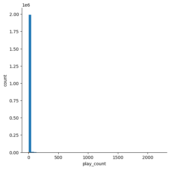
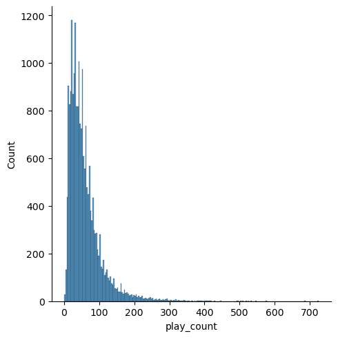
From this distribution plot, we can see that the number of songs played by each user (lets call it user interactions) is heavily right skewed. There are many (thousands) users who have only listened to a few songs, so any matrix I build from this data will be extremely sparse. Next I reduce the skew in the play_counts by filtering out users who have less than a minimum (I settled on 90) number of total plays. These are users that there is very little preference data for. Plotting the distriution of ‘play_count’ after filtering:
| Column | Non-Null | Count | Dtype | |
|---|---|---|---|---|
| 0 | user_id | 1224498 | non-null | object |
| 1 | song_id | 1224498 | non-null | object |
| 2 | title | 1224498 | non-null | object |
| 3 | release | 1224498 | non-null | object |
| 4 | artist_name | 1224498 | non-null | object |
| 5 | year | 1224498 | non-null | int64 |
| 6 | play_count | <1224498 | non-null | int64 |
Filtering out less active users has decreased the imbalance somewhat. The distribution is still heavily right skewed in the above plot, but the class imbalance has been reduced by a factor of 5 (y limit is 1200 instead of 7000). This has also decreased the size of the dataset to 1.2 million records down from 2 million.
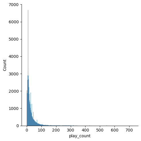
This is still not good enough, so I continue to decrease the sparcity and imbalance of the data by filtering out any user/song records that have a play count less than 6. There are many more songs that users have only listened to 1 or a few times. I want to recommend highly rated songs, so I am going to get rid of these songs with low interactions and assume they are uninteracted with ‘not-liked’.
| Column | Non-Null | Count | Dtype | |
|---|---|---|---|---|
| 0 | user_id | 185694 | non-null | object |
| 1 | song_id | 185694 | non-null | object |
| 2 | title | 185694 | non-null | object |
| 3 | release | 185694 | non-null | object |
| 4 | artist_name | 185694 | non-null | object |
| 5 | year | 185694 | non-null | int64 |
| 6 | play_count | <185694 | non-null | int64 |
This last filtering step dramatically reduced the size of the dataset by 85%, this will speed up processing times for the models and also make the predictions more accurate by reducing the class imbalance. Finally, I filter out all songs that have less than 20 user interactions:
| Column | Non-Null | Count | Dtype | |
|---|---|---|---|---|
| 0 | user_id | 124147 | non-null | object |
| 1 | song_id | 124147 | non-null | object |
| 2 | title | 124147 | non-null | object |
| 3 | release | 124147 | non-null | object |
| 4 | artist_name | 124147 | non-null | object |
| 5 | year | 124147 | non-null | int64 |
| 6 | play_count | <124147 | non-null | int64 |
With these filtering steps, I have reduced the class imbalance, decreased the size of the dataset to make models and gridsearch more tracteable, and I have decreased the extreme sparcity of our resulting recommendations matrices. Now I am going to apply a threshhold limit to further reduce class imblance and the play_count range, and then apply a min max scalar to standardize the play_counts so I can effectively use them as a proxy for a 1-10 rating.
Clipping and Scaling play_count:
Because there are very few users who have listened to a song more than 25 times, I will set a threshold at 25 plays. I dont want to drop records with more than 25 plays because this is important information on users likes, So I will clip anything > 25 to 25 and then apply a MinMaxScalar function from the sklearn package to scale the playcounts from 1-10.
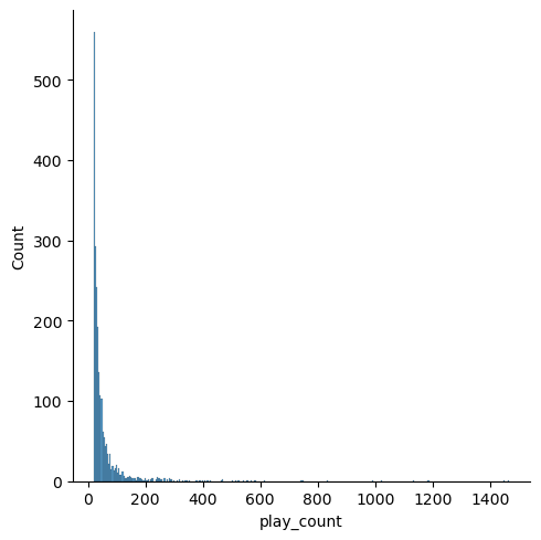
Distribution plot after filtering:
Distribution plot after scaling:
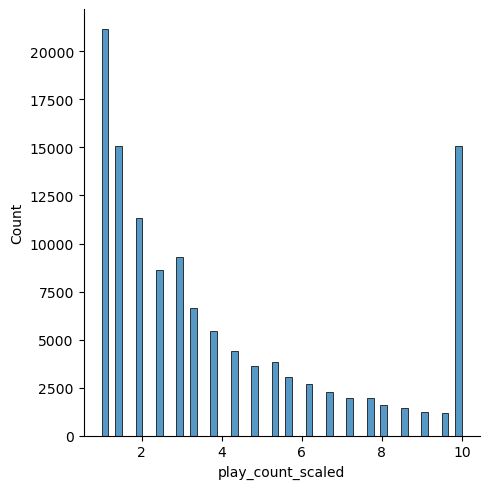
My final play_counts, filtered, clipped, and scaled look pretty good. The class imbalance between the left side of the X axis and the higher play_counts has been reduced, The play_counts are scaled from 1-10, and I have kept the records containing the highest ratings as 10’s.
(121900, 8)
The final dataset has 121,900 records. This is a much more maneagable number of records for training and testing models. After previous iterations of testing the filtering, I had dropped over 90% of the songs so the final recommendations that were being made were not diverse and nearly the same for every user. So Im going to continue EDA and take a look at the filtered dataset to make sure the user/song diversity is still good…
Exploratory Data Analysis Continued…
Checking the total number of unique users, songs, artists in the data
Total number of unique user id
Number of unique USERS = 19212
Total number of unique song id
Number of unique SONGS = 2210
Total number of unique artists
Number of unique artists = 1194
Observations and Insights:
- There are 19212 unique users remaining in the dataset after filtering
- There are 2210 unique songs remaining in the dataset after filtering
- There are 1194 Unique artists remaining in the dataset after filtering
- This looks like a great balance, we have filtered out rare users and songs but retained many different users and we have a diversity of songs and artists.
Let’s find out about the most interacted songs and interacted users
Most interacted songs
| song_id | play_count | |
|---|---|---|
| 138 | SOBONKR12A58A7A7E0 | 1466 |
| 80 | SOAUWYT12A81C206F1 | 1445 |
| 1624 | SOSXLTC12AF72A7F54 | 1186 |
| 478 | SOFRQTD12A81C233C0 | 1133 |
| 88 | SOAXGDH12A8C13F8A1 | 1024 |
| 357 | SOEGIYH12A6D4FC0E3 | 993 |
| 1188 | SONYKOW12AB01849C9 | 831 |
| 1901 | SOWCKVR12A8C142411 | 748 |
| 1343 | SOPUCYA12A8C13A694 | 744 |
| 647 | SOHTKMO12AB01843B0 | 616 |
Most interacted users
| user_id | play_count | |
|---|---|---|
| 5683 | 4be305e02f4e72dad1b8ac78e630403543bab994 | 106 |
| 766 | 0a4c3c6999c74af7d8a44e96b44bf64e513c0f8b | 82 |
| 827 | 0b19fe0fad7ca85693846f7dad047c449784647e | 81 |
| 8262 | 6d625c6557df84b60d90426c0116138b617b9449 | 74 |
| 16334 | da3890400751de76f0f05ef0e93aa1cd898e7dbc | 69 |
| 7930 | 695179610d0b1fbb9d66267a3bd24946617af7fb | 67 |
| 17477 | e9a7dba8248ced646ea192016660e3c9056c0d03 | 66 |
| 2996 | 283882c3d18ff2ad0e17124002ec02b847d06e9a | 65 |
| 5405 | 48567d388c6a7dda0e9d0a7b6648bdb42440475c | 65 |
| 10463 | 8c78c69701072e204f4340ca4d6ee44fe39e40cc | 64 |
Observations and Insights:
- The most interacted song is ‘SOBONKR12A58A7A7E0’ which has been interacted with by 1466 different users
- The most active user is ‘4be305e02f4e72dad1b8ac78e630403543bab994’, they have listened to 106 different songs
Songs played in a year
| 0 | 49 | 48 | 47 | 46 | 43 | 45 | 50 | 41 | 42 | ... | 17 | 21 | 7 | 6 | 3 | 5 | 12 | 1 | 2 | 4 | |
|---|---|---|---|---|---|---|---|---|---|---|---|---|---|---|---|---|---|---|---|---|---|
| year | 0 | 2009 | 2008 | 2007 | 2006 | 2003 | 2005 | 2010 | 2001 | 2002 | ... | 1977 | 1981 | 1967 | 1966 | 1962 | 1965 | 1972 | 1958 | 1960 | 1963 |
| play_count | 26580 | 12782 | 10616 | 7499 | 6693 | 5718 | 4861 | 4617 | 4316 | 4147 | ... | 151 | 145 | 137 | 134 | 113 | 110 | 77 | 66 | 62 | 61 |
2 rows × 51 columns
Text(0, 0.5, 'number of releases')
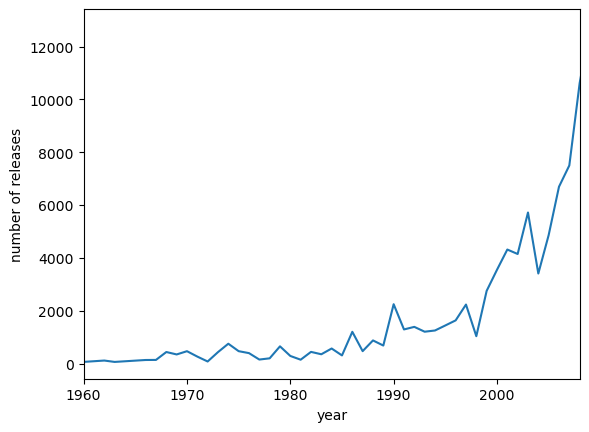
Observations and Insights:
- It is not clear whether the ‘year’ feature is, but it is most likely the year a song/album was released.
- We can clearly see that there in an increasing trend from 1960-2008 in the number of songs released
- This makes sense as there are more people, more artists, and musical equiptment, recording equiptment, and streaming platforms have made it easier to produce music
Now I apply different algorithms to build a recommendation system.
Building a baseline popularity-based recommendation system
In this basic recommendation system, I take the count and sum of play counts of the songs and build the popularity recommendation system based on the sum of play counts (For the full code check out the Github Link at the bottom of the page). The rank based recommender function is:
Here is the output after running the popularity-based RS on the filtered dataset:
| title | artist_name | |
|---|---|---|
| 0 | 221 | keller williams |
| 1 | Call It Off (Album Version) | Tegan And Sara |
| 2 | Clara meets Slope - Hard To Say | Clara Hill |
| 3 | Kelma | Rachid Taha |
| 4 | Numb (Album Version) | Disturbed |
| 5 | Voices On A String (Album Version) | Thursday |
| 6 | What If I Do? | Foo Fighters |
| 7 | Encore Break | Pearl Jam |
| 8 | Reign Of The Tyrants | Jag Panzer |
| 9 | Dance_ Dance | Fall Out Boy |
Collaborative Filtering, Matrix Factorization, and Clustering based recommendation sytems
Before running the following recommendation systems, I developed several functions for calculating metrics to evaluate the models. The metrics I used are Root Mean Squared Error, Mean Average Error, Precision, Recall, and F1.
I then split the data into a train and test set (Link to full code is at the bottom of the page). Also, to build the user-user-similarity-based and subsequent models I used the “surprise” library from Python.
User User Similarity-Based Collaborative Filtering Metrics
The code for implementing the user-user similarity matrix with base settings is:
Result:
RMSE: 3.1852
MAE:  2.5755
  algorithm      rmse       mae  precision  recall  f1_score  popularity
0  KNNbasic  3.185239  2.575525      0.682   0.772     0.724        24.3
Observations and Insights:
For the untuned User-user similarity-based model,
- The RMSE is 3.18
- The MAE is 2.57
- The f1 score is 0.72
- The average popularity of recommended songs is 24.3
predictions using knn.KNNBasic for user 6ccd111af9b4baa497aacd6d1863cbf5a141acc6:
- prediction for Red Dirt Road by Brooks and Dunn: r_ui = 10.00 est = 3.97
- predictions for Till I collapse by Eminem and Nate Dogg: r_ui = 1.00 est = 3.74
- prediction for SOTTGXB12A6701FA0B by Phoenix (other pheonix songs are 7.6): r_ui = None est = 3.45
Observations and Insights:
- For the song the user has seen with a rating of 10, the model predicted a rating of 3.97
- For the song the user has seen with a rating of 1, the model predicted a rating of 3.74
- For the unheard songs by the user, the model predicted 3.45
- The user-user similarity-based collaborative filtering method has good RMSE, MAE and f1_score, but…
- The user-user model isnt predicting ratings very well
- All three songs have similar predicted ‘ratings’ for this user
Next, I tuned the model using GridSearchCV to try to improve the model performance.
The metrics after tuning are:
2.8805243519619927
{'k': 50, 'min_k': 9, 'sim_options': {'name': 'msd', 'user_based': True}}

RMSE: 2.8309
MAE:  2.2550
        algorithm      rmse       mae  precision  recall  f1_score  popularity
0        KNNbasic  3.185239  2.575525      0.682   0.772     0.724        24.3
1  KNNbasic_tuned  2.830942  2.254989      0.698   0.799     0.745        64.9
Observations and Insights:
After tuning the user-user model,
- The RMSE has decreased over the untuned model
- The MAE has also decreased
- The f1 score has increased
- The popularity of recommended songs has increased
predictions using knn.KNNBasic tuned for user 6ccd111af9b4baa497aacd6d1863cbf5a141acc6:
- prediction for Red Dirt Road by Brooks and Dunn: r_ui = 10.00 est = 8.95
- predictions for Till I collapse by Eminem and Nate Dogg: r_ui = 1.00 est = 3.14
- prediction for SOTTGXB12A6701FA0B by Phoenix (other pheonix songs are 7.6): r_ui = None est = 3.38
Observations and Insights:
- The model is predicting a rating of 8.95 for the song the user has heard and rated a 10, this is very good.
- The model is predicting a rating of 3.14 for the song the user has heard and rated a 1, this is not bad.
- The model is rating the unheard song 3.38.
- It seems that tuning the model has improved its ability to predict ratings
Finally, because more ‘popular’ songs are more likely to be ‘liked’, I adjust the tuned recommendations by using a custom script to weight recommendations by the number of plays. The final, weighted, recommednations from the User-User similarity-based recommendation system for user ‘6ccd111af9b4baa497aacd6d1863cbf5a141acc6’ are:
| title | artist_name | count_plays | predicted_interaction | corrected_ratings | |
|---|---|---|---|---|---|
| 0 | Clara meets Slope - Hard To Say | Clara Hill | 89 | 9.205088 | 9.099088 |
| 1 | Numb (Album Version) | Disturbed | 68 | 8.825430 | 8.704162 |
| 2 | When You're Gone | Avril Lavigne | 76 | 8.568666 | 8.453958 |
| 3 | #40 | DAVE MATTHEWS BAND | 72 | 8.503340 | 8.385488 |
| 4 | Speechless (Album Version) | The Veronicas | 45 | 8.512847 | 8.363776 |
| 5 | XRDS | Covenant | 51 | 8.475145 | 8.335117 |
| 6 | (iii) | The Gerbils | 88 | 8.352223 | 8.245623 |
| 7 | Modern world | Modern Lovers | 51 | 8.274458 | 8.134430 |
| 8 | The Memory Remains | Metallica / Marianne Faithfull | 94 | 8.209485 | 8.106343 |
| 9 | Sunburn | Muse | 15 | 8.156890 | 7.898691 |
Observations and Insights:
- I predicted 10 songs for the user ‘6d625c6557df84b60d90426c0116138b617b9449’ with the user-user collaborative filtering method
- Some of the songs that are recommended to the user have a predicted rating close to 10, this is very good.
- Evaluating the tuned and untuned models, the tuned model has improved performance based on the evaluation metrics I chose.
Item-Item Similarity-based collaborative filtering recommendation system
Metrics of the item-item model compared to user-user
RMSE: 2.9990
MAE:  2.2550
        algorithm      rmse       mae  precision  recall  f1_score  popularity
0        KNNbasic  3.185239  2.575525      0.682   0.772     0.724        24.3
1  KNNbasic_tuned  2.830942  2.254989      0.698   0.799     0.745        64.9
2   KNNbasic_item  2.998977  2.254952      0.658   0.736     0.695        25.1
Observations and Insights:
- The RMSE for the item-item model is 2.99
- The item-item collaborative filtering model has nearly the the same MAE as the tuned user-user model
- the f1 score is 0.695
- The popularity of recommended songs is 25
predictions using knn.KNNBasic_item for user 6ccd111af9b4baa497aacd6d1863cbf5a141acc6:
- prediction for Red Dirt Road by Brooks and Dunn: r_ui = 10.00 est = 4.40
- predictions for Till I collapse by Eminem and Nate Dogg: r_ui = 1.00 est = 4.44
- prediction for SOTTGXB12A6701FA0B by Phoenix (other pheonix songs are 7.6): r_ui = None est = 4.72
Observations and Insights:
- The model is predicting 4.4 for the heard song that had rating of 10
- The model is predicting 4.44 for the heard song that had rating of 1
- The model is predicting 4.72 for the unheard song
- Overall, the prediction of ratings is poor compaired to the tuned user-user model
Next, I ran GridsearchCV to to search for the optimal hyperparameters to tune the item-item model with. The optimal hyperparameter settings after running GridSearch are:
2.9243151529965794
{'k': 50, 'min_k': 3, 'sim_options': {'name': 'cosine', 'user_based': False}}
Model Metrics for item-item model after rerunning with the tuned paramters
RMSE: 2.9040
MAE:  2.3017
             algorithm      rmse       mae  precision  recall  f1_score  \
0             KNNbasic  3.185239  2.575525      0.682   0.772     0.724
1       KNNbasic_tuned  2.830942  2.254989      0.698   0.799     0.745
2        KNNbasic_item  2.998977  2.254952      0.658   0.736     0.695
3  KNNbasic_item_tuned  2.903997  2.301706      0.688   0.785     0.733
predictions using knn.KNNBasic_item tuned for user 6ccd111af9b4baa497aacd6d1863cbf5a141acc6:
- prediction for Red Dirt Road by Brooks and Dunn: r_ui = 10.00 est = 4.61
- predictions for Till I collapse by Eminem and Nate Dogg: r_ui = 1.00 est = 4.44
- prediction for SOTTGXB12A6701FA0B by Phoenix (other pheonix songs are 7.6): r_ui = None est = 4.72
Observations and Insights:
- The RMSE decreased slightly after tuning
- The MAE has increased slightly
- The f1 score increased
- The popularity is the same
- similar to the untuned item-item model, our predictions are rather poor
- In general, the predicted ratings of all the songs are about the same as the untuned model
- Given that all of these songs are quite different, these predictions may not reflect the users actually taste.
The final, weighted, recommendations from the Item-Item similarity-based recommendation system for user ‘6ccd111af9b4baa497aacd6d1863cbf5a141acc6’ are:
| title | artist_name | count_plays | predicted_interaction | corrected_ratings | |
|---|---|---|---|---|---|
| 0 | Ni Tú Ni Nadie (Versión Demo) | Alaska Y Dinarama | 31 | 10.000000 | 9.820395 |
| 1 | My Perfect Cousin | The Undertones | 21 | 9.842105 | 9.623887 |
| 2 | Walk On Water Or Drown (Album) | Mayday Parade | 24 | 9.684211 | 9.480086 |
| 3 | Docking Bay 94 | The Alter Boys | 25 | 9.661287 | 9.461287 |
| 4 | Waters Of Nazareth (album version) | Justice | 29 | 9.210526 | 9.024831 |
| 5 | Valentine | Justice | 24 | 8.934211 | 8.730086 |
| 6 | Please_ Before I Go | Derek Webb | 32 | 8.905551 | 8.728775 |
| 7 | Hitsville U.K. | The Clash | 25 | 8.421053 | 8.221053 |
| 8 | Go Places | The New Pornographers | 20 | 8.342105 | 8.118498 |
| 9 | Uptown | Drake / Bun B / Lil Wayne | 24 | 8.061607 | 7.857483 |
Observations and Insights:
- Interestingly, the item-item model recommends a completely different top 10 songs than the user-user model
Model Based Collaborative Filtering - Matrix Factorization
Model-based Collaborative Filtering is a personalized recommendation system, the recommendations are based on the past behavior of the user and it is not dependent on any additional information. It uses latent features to find recommendations for each user. Here I am using Singular Value Decomposition (SVD) method from the Suprise library, and calculate the metrics after running the base model with default settings:
RMSE: 2.7215
MAE:  2.1682
             algorithm      rmse       mae  precision  recall  f1_score  \
0             KNNbasic  3.185239  2.575525      0.682   0.772     0.724
1       KNNbasic_tuned  2.830942  2.254989      0.698   0.799     0.745
2        KNNbasic_item  2.998977  2.254952      0.658   0.736     0.695
3  KNNbasic_item_tuned  2.903997  2.301706      0.688   0.785     0.733
4                  SVD  2.721453  2.168153      0.696   0.798     0.744
predictions using SVD tuned for user 6ccd111af9b4baa497aacd6d1863cbf5a141acc6:
- prediction for Red Dirt Road by Brooks and Dunn: r_ui = 10.00 est = 8.95
- predictions for Till I collapse by Eminem and Nate Dogg: r_ui = 1.00 est = 2.06
- prediction for SOTTGXB12A6701FA0B by Phoenix (other pheonix songs are 7.6): r_ui = None est = 5.39
Observations and Insights:
- The SVD model has the best RMSE and MAE of any models yet
- The f1 score is higher than any other untuned models
- The popularity of recommended songs is far higher than the other models
- The predictions for the heard song with rating 10 is 8.95
- The predictions for the heard song with rating 1 is 2.06
- The prediciton for the unheard song is 5.39
- These are the most accurate predictions yet of any of the models
Improving matrix factorization based recommendation system by tuning its hyperhyperparameters
To tune the SVD model, first I run a factor checking function that plots the RMSE based on a range of latent features.
Here is the plot for this data run for 100 features:
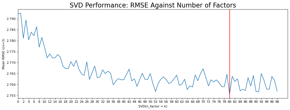
According to the figure, there is a decreasing trend of better performance with higher k. The lowest RMSE is achieved when k is 80. However, it is worth mentioning that k = 52 and >84 are also good. The result suggests a range of values which can be used in GridSearchCV()for hyperparameter tunning. Next I ran GridSearchCV to find the optimal hyperparameter settings. The hyperparameter settings for the model that reduced RMSE the most are:
2.7097656150739744
{'n_epochs': 30, 'lr_all': 0.01, 'reg_all': 0.4, 'n_factors': 80}
Model Metrics for Matrix Factorization (SVD) method after rerunning with the tuned paramters
RMSE: 2.6736
MAE:  2.1434
             algorithm      rmse       mae  precision  recall  f1_score  \
0             KNNbasic  3.185239  2.575525      0.682   0.772     0.724
1       KNNbasic_tuned  2.830942  2.254989      0.698   0.799     0.745
2        KNNbasic_item  2.998977  2.254952      0.658   0.736     0.695
3  KNNbasic_item_tuned  2.903997  2.301706      0.688   0.785     0.733
4                  SVD  2.721453  2.168153      0.696   0.798     0.744
5            SVD_tuned  2.673590  2.143426      0.694   0.799     0.743
predictions using SVD tuned tuned for user 6ccd111af9b4baa497aacd6d1863cbf5a141acc6:
- prediction for Red Dirt Road by Brooks and Dunn: r_ui = 10.00 est = 8.22
- predictions for Till I collapse by Eminem and Nate Dogg: r_ui = 1.00 est = 4.71
- prediction for SOTTGXB12A6701FA0B by Phoenix (other pheonix songs are 7.6): r_ui = None est = 5.13
Observations and Insights:
- The tuned SVD model has a slightly lower RMSE and MAE than the base SVD model
- the f1_score of the the tuned SVD model increased .01
- The popularity of the tuned model dropped significantly
- The popularity of the base model may have been affected by a single highly rated song.
- The predictions for the heard song with rating 10 is about the same as the untuned model
- the prediction for the heard song with rating 1 came up a bit to 2
- In general the predicted ratings are much better than the non matrix factorization models, but tuning the SVD model did not improve performance much if at all.
Since the untuned SVD model had predictions that were the closest to the users actually play counts, Im going to look at the weighted recommendations for both the default and tuned SVD algorithms. The final, weighted, recommendations from default SVD matrix factorization algorithm for user ‘6ccd111af9b4baa497aacd6d1863cbf5a141acc6’ are:
| title | artist_name | count_plays | predicted_interaction | corrected_ratings | |
|---|---|---|---|---|---|
| 0 | Catch You Baby (Steve Pitron & Max Sanna Radio... | Lonnie Gordon | 616 | 10.000000 | 9.959709 |
| 1 | Clara meets Slope - Hard To Say | Clara Hill | 89 | 9.879379 | 9.773379 |
| 2 | Make Her Say | Kid Cudi / Kanye West / Common | 156 | 9.186673 | 9.106609 |
| 3 | Something (Album Version) | Jaci Velasquez | 95 | 8.532769 | 8.430171 |
| 4 | Electric Feel | MGMT | 179 | 8.380396 | 8.305653 |
| 5 | He's A Pirate | Klaus Badelt | 20 | 8.514556 | 8.290949 |
| 6 | 221 | keller williams | 51 | 8.379492 | 8.239464 |
| 7 | Gunn Clapp | O.G.C. | 86 | 8.313128 | 8.205295 |
| 8 | Call It Off (Album Version) | Tegan And Sara | 66 | 8.098702 | 7.975610 |
| 9 | Girls | Death In Vegas | 25 | 8.072738 | 7.872738 |
And the Tuned recommendations:
| title | artist_name | count_plays | predicted_interaction | corrected_ratings | |
|---|---|---|---|---|---|
| 0 | False Pretense | The Red Jumpsuit Apparatus | 21 | 7.612781 | 7.394563 |
| 1 | Sorrow (1997 Digital Remaster) | David Bowie | 77 | 6.734795 | 6.620835 |
| 2 | I'd Hate To Be You When People Find Out What T... | Mayday Parade | 21 | 6.831190 | 6.612972 |
| 3 | Recado Falado (Metrô Da Saudade) | Alceu Valença | 143 | 6.648431 | 6.564807 |
| 4 | Q-Ball | Brotha Lynch Hung | 33 | 6.705204 | 6.531126 |
| 5 | Underground | Eminem | 24 | 6.631778 | 6.427654 |
| 6 | Cold Blooded (Acid Cleanse) | The fFormula | 38 | 6.565968 | 6.403747 |
| 7 | Walk Through Hell (featuring Max Bemis Acousti... | Say Anything | 31 | 6.578550 | 6.398944 |
| 8 | Night Village | Deep Forest | 20 | 6.575026 | 6.351420 |
| 9 | Drive | Savatage | 24 | 6.539166 | 6.335042 |
Observations and Insights:
- The recommended songs from the tuned svd model are much different than the untuned svd model
- In general, it seems that the tuned model is recommending less popular songs
Cluster Based Recommendation System
In clustering-based recommendation systems, we explore the similarities and differences in people’s tastes in songs based on how they rate different songs. We cluster similar users together and recommend songs to a user based on play_counts from other users in the same cluster. After running the Coclustering method with default settings, the metrics compared to the other models are:
RMSE: 2.9591
MAE:  2.2116
             algorithm      rmse       mae  precision  recall  f1_score  \
0             KNNbasic  3.185239  2.575525      0.682   0.772     0.724
1       KNNbasic_tuned  2.830942  2.254989      0.698   0.799     0.745
2        KNNbasic_item  2.998977  2.254952      0.658   0.736     0.695
3  KNNbasic_item_tuned  2.903997  2.301706      0.688   0.785     0.733
4                  SVD  2.721453  2.168153      0.696   0.798     0.744
5            SVD_tuned  2.673590  2.143426      0.694   0.799     0.743
6         CoClustering  2.959111  2.211564      0.622   0.666     0.643
predictions using SVD tuned tuned for user 6ccd111af9b4baa497aacd6d1863cbf5a141acc6:
- prediction for Red Dirt Road by Brooks and Dunn: r_ui = 10.00 est = 4.71
- predictions for Till I collapse by Eminem and Nate Dogg: r_ui = 1.00 est = 4.00
- prediction for SOTTGXB12A6701FA0B by Phoenix (other pheonix songs are 7.6): r_ui = None est = 3.17
Observations and Insights:
- The clustering model has an RMSE of 2.9 and MAE of 2.2
- The f1 score is .643
- Overal the clustering metrics are performing similarly slightly poorer compared to other models
- The predicted rating for the song with rating 10 is 4.71
- The predictions for the other heard song with raitng 1 is 4
Next, I run GridsearchCV on the clustering-based recommendation system to tune its hyper-hyperparameters. The optimal hyperhyperparameters suggested by the search are:
3.0094114249385258
{'n_cltr_u': 3, 'n_cltr_i': 3, 'n_epochs': 40}
The model metrics after rerunning coclustering with the tuned hyperparamters
RMSE: 2.9613
MAE:  2.2139
             algorithm      rmse       mae  precision  recall  f1_score  \
0             KNNbasic  3.185239  2.575525      0.682   0.772     0.724
1       KNNbasic_tuned  2.830942  2.254989      0.698   0.799     0.745
2        KNNbasic_item  2.998977  2.254952      0.658   0.736     0.695
3  KNNbasic_item_tuned  2.903997  2.301706      0.688   0.785     0.733
4                  SVD  2.721453  2.168153      0.696   0.798     0.744
5            SVD_tuned  2.673590  2.143426      0.694   0.799     0.743
6         CoClustering  2.959111  2.211564      0.622   0.666     0.643
7   CoClustering_tuned  2.961292  2.213922      0.622   0.666     0.643
predictions using SVD tuned tuned for user 6ccd111af9b4baa497aacd6d1863cbf5a141acc6:
- prediction for Red Dirt Road by Brooks and Dunn: r_ui = 10.00 est = 4.7
- predictions for Till I collapse by Eminem and Nate Dogg: r_ui = 1.00 est = 3.99
- prediction for SOTTGXB12A6701FA0B by Phoenix (other pheonix songs are 7.6): r_ui = None est = 3.23
Observations and Insights:
- Tuning the clustering model has not improved it, or only marginally
- The prediction for the heard song with rating 10 is 4.7
The final, weighted, recommendations from the tuned coclustering algorithm for user ‘6ccd111af9b4baa497aacd6d1863cbf5a141acc6’ are:
| title | artist_name | count_plays | predicted_interaction | corrected_ratings | |
|---|---|---|---|---|---|
| 0 | Love Is Gone (Original Mix) | David Guetta - Joachim Garraud - Chris Willis | 20 | 8.561523 | 8.337917 |
| 1 | Cold Blooded (Acid Cleanse) | The fFormula | 38 | 8.275809 | 8.113588 |
| 2 | The World Is Mine | David Guetta | 21 | 8.056761 | 7.838544 |
| 3 | What Is Light? Where Is Laughter? (Album Version) | Twin Atlantic | 20 | 7.872448 | 7.648841 |
| 4 | Kelma | Rachid Taha | 58 | 7.642269 | 7.510962 |
| 5 | Love Is Not A Fight | Warren Barfield | 36 | 7.561523 | 7.394857 |
| 6 | I Wonder Why | Dion & The Belmonts | 41 | 7.517873 | 7.361699 |
| 7 | Hasta siempre | Varios | 20 | 7.552595 | 7.328988 |
| 8 | Numb (Album Version) | Disturbed | 68 | 7.418666 | 7.297398 |
| 9 | 221 | keller williams | 51 | 7.411147 | 7.271119 |
Observations and Insights:
- Ther top 10 recommended songs are similar to the user-user and SVD models
Content Based Recommendation System
So far I have only used the play_count of songs to find recommendations but there are other information/features on songs as well, and these features can be used to increase the personalization of the recommendation system. For example, we can use the artist name and album title to recommend songs to users from artists/albums they like but songs they have not heard yet. We can also include the year the song was released and recommend music from the same time period. Here are the main functions I used for the content model:
Before Running any of the content based models, I preprocessed the text data by tolkenizing it with natural language processing methods that come standard in the NLTK package. First, I coded the year column into text:
| song_id | artist_name | release | year | year_text | |
|---|---|---|---|---|---|
| 0 | SODGVGW12AC9075A8D | Justin Bieber | My Worlds | 2010 | twothousandtens |
| 1 | SODGVGW12AC9075A8D | Justin Bieber | My World 2.0 | 2010 | twothousandtens |
| 2 | SOEPZQS12A8C1436C7 | Deadmau5 | Ghosts 'n' Stuff | 2009 | twothousandzeros |
| 3 | SOGDDKR12A6701E8FA | Eminem / Hailie Jade | The Eminem Show | 2006 | twothousandzeros |
| 4 | SOWGXOP12A6701E93A | Eminem | Without Me | 2002 | twothousandzeros |
Then I combined all of the text features into a single column ‘text’:
| year_text | text | |
|---|---|---|
| song_id | ||
| SODGVGW12AC9075A8D | twothousandtens | Justin Bieber My Worlds twothousandtens |
| SODGVGW12AC9075A8D | twothousandtens | Justin Bieber My World 2.0 twothousandtens |
| SOEPZQS12A8C1436C7 | twothousandzeros | Deadmau5 Ghosts 'n' Stuff twothousandzeros |
| SOGDDKR12A6701E8FA | twothousandzeros | Eminem / Hailie Jade The Eminem Show twothousa... |
| SOWGXOP12A6701E93A | twothousandzeros | Eminem Without Me twothousandzeros |
I then calculated a tf-idf matrix and calculated the cosign similarity.
The Recommendations using this method are:
| title | artist_name | count_plays | predicted_interaction | corrected_ratings | |
|---|---|---|---|---|---|
| 0 | Cats In The Cradle | Ugly Kid Joe | 30 | 7.789474 | 7.606899 |
| 1 | Cold Blooded (Acid Cleanse) | The fFormula | 38 | 7.000000 | 6.837779 |
| 2 | Hold Me_ Thrill Me_ Kiss Me_ Kill Me | U2 | 33 | 6.770725 | 6.596648 |
| 3 | Twilight Galaxy | Metric | 28 | 6.696697 | 6.507715 |
| 4 | Last Nite | The Strokes | 21 | 6.724206 | 6.505988 |
| 5 | The Calculation (Album Version) | Regina Spektor | 44 | 6.636842 | 6.486086 |
| 6 | Mansard Roof (Album) | Vampire Weekend | 26 | 6.587426 | 6.391310 |
| 7 | Face To Face | Daft Punk | 32 | 6.525241 | 6.348465 |
| 8 | Injection | Rise Against | 23 | 6.485387 | 6.276872 |
| 9 | Chinese | Lily Allen | 14 | 6.092105 | 5.824844 |
Observations and Insights:
- This is excellent, we are recommending songs by the same artists/albums the user has likes and adding in some weight for the decade of the users song preferences.
- We are also ranking the recommendations based on song popularity, so more listened to songs by other users will be weighted heavier for this user
hybrid recommendation system
I have explored five different recommender methods (six if you include the popularity-based method) for recommending songs to a user in a personalized way. This is all well and good, but how do we know which method is recommending songs the user will actualy listen to? As an avid listener of music, is it not also true that a users preferences can change, and may change drastically during the day or from day to day? It also seems that the models we have presented so far sometimes recommend similar songs, but other models are drastically different as in the item-item recommendations and content based recommendations. In this section, I build a hybrid recommender system which takes into account recommendations from multiple models, applys weights based on which models we want to be most represented in the results, and then provides a ‘hybrid’ recommendation.
In my hybrid system, I fit models and make predictions by combing two of the previously evaluated models:
- SVD (default settings)
- User-User collaborative Filtering (tuned)
I chose these two models because both had the best F1_scores metrics, both had fairly good predictions, and both recommended markedly different songs. I then add in a subset of recommendations from the content-based filtering method to increase the ‘familiarity’ for the user of the recommended songs/artists. This will hopefully provide a highly personalized recommendation for a user with a balance of new songs and familiar artists to give choices based on potential dynamic user preferences. I also evaluated the performance of different weight combinations using the hold-out set. For example, we can try different combinations of wA and wB for the SVD and User-User model combination, ranging from (0.1, 0.9) to (0.9, 0.1), and compute their respective RMSE scores:
RMSE: 2.7976
MAE:  2.2302
Weight combination (0.1, 0.9): RMSE = 2.7976, MAE = 2.2302
RMSE: 2.7495
MAE:  2.1971
Weight combination (0.3, 0.7): RMSE = 2.7495, MAE = 2.1971
RMSE: 2.7186
MAE:  2.1749
Weight combination (0.5, 0.5): RMSE = 2.7186, MAE = 2.1749
RMSE: 2.7057
MAE:  2.1634
Weight combination (0.7, 0.3): RMSE = 2.7057, MAE = 2.1634
RMSE: 2.7110
MAE:  2.1619
Weight combination (0.9, 0.1): RMSE = 2.7110, MAE = 2.1619
Observations and Insights:
- there is not much difference in RMSE for the different combinations of model weights
- The ‘best’ weight combination is SVD .7 - collaborative filtering .3
Conclusion and Recommendations
1. Comparison of various techniques and their relative performance based on chosen Metric (Measure of success):
- In General the Method 2 dataset had better MSE and MAE than the method 1 dataset, but the Method 1 dataset had better f1_score and the predictions for listened to songs were closer to the actual playcounts
- The SVD and user-user based models performed the best according to RMSE, MAE, and f1
- The item-item model recommended different songs that the SVD, clustering, and user-user
- In general, tuning the models did improve their performance, however it became clear that one of the biggest effects on model performance is the data going into the model.
- The Content based recommender system, just based on artist name, album title and year does a decent job of recommending artists the user likes, and songs from albums the user has listened to.
- Many of the songs in the SVD,clustering, collaboritive filtering recommendations were not artists in the users top listened artist/song list, therefore I added the Content Based Recommendations into the hybrid recommender system.
- I chose to tune my hybrid recommendation system using SVD with default settings because it was the best performing model, and user-user collaborative Filtering model. Combining these added more potential song diversity that might align with the user preferences into the final recommendation.
- I also added content-based recommendations into the hybrid model for ‘familiarity’
- There is room for improvement in the performance of the models and final recommender system:
- more features such as genre, loudness, danceability, and lyrics could be added as features to improve Content based recommendations
- Further improvement could be made on filtering/scaling the play_counts to achieve better predictions
- A different approach could be tried, such as Neural Networks
2. Refined insights:
- The impact of the Y variable - in this case play_count - cannot be understated.
- The distribution and scarcity in the play_counts, and how I chose to filter and transform it had large impacts on the model performance
- The Content-based recommender system, although perhaps the ‘simplist’ of the models besides the popularity based recommender system, performs predictably and precisely recommends songs based on content
- matrix factorization outperformed other models. It runs quickly, and while it has only marginally better performace metrics than other collaborative or cluster-based models, its predictions were the closest to actual.
- The metrics you choose to assess model performance with are extremely important. depending on the metrics you choose, they can change the decisions you make about models and recommendations.
3. Proposal for the final solution design:
- I am proposing the hybrid recommender system I built be adopted. It provides a good balance of artists/albums the user is known to like, but may not have listened to other songs of, and new content recommended by usesr-user collaborative filtering and matrix factorization,
- In short, it is highly personalized!
- This hybrid recommender system could be adjusted and improved further based on more features for content-based recommending or alternative compositions of models/weights
Final 10 song recommendation for user 6d625c6557df84b60d90426c0116138b617b9449:
| title | artist_name | count_plays | predicted_interaction | corrected_ratings | |
|---|---|---|---|---|---|
| 0 | Clara meets Slope - Hard To Say | Clara Hill | 89 | 9.677092 | 9.571092 |
| 1 | Catch You Baby (Steve Pitron & Max Sanna Radio... | Lonnie Gordon | 616 | 8.470891 | 8.430600 |
| 2 | Make Her Say | Kid Cudi / Kanye West / Common | 156 | 7.772713 | 7.692649 |
| 3 | Cats In The Cradle | Ugly Kid Joe | 30 | 7.789474 | 7.606899 |
| 4 | Recado Falado (Metrô Da Saudade) | Alceu Valença | 143 | 7.642525 | 7.558901 |
| 5 | #40 | DAVE MATTHEWS BAND | 72 | 7.661807 | 7.543956 |
| 6 | Walk Through Hell (featuring Max Bemis Acousti... | Say Anything | 31 | 7.678929 | 7.499324 |
| 7 | Eternal Flame (Single Version) | Atomic Kitten | 49 | 7.411352 | 7.268495 |
| 8 | Cold Blooded (Acid Cleanse) | The fFormula | 38 | 7.000000 | 6.837779 |
| 9 | Hold Me_ Thrill Me_ Kiss Me_ Kill Me | U2 | 33 | 6.770725 | 6.596648 |
References
- Thierry Bertin-Mahieux, Daniel P.W. Ellis, Brian Whitman, and Paul Lamere. The Million Song Dataset. In Proceedings of the 12th International Society for Music Information Retrieval Conference (ISMIR 2011), 2011.