Overview:
This analysis was part of my submission for the Great Learning Spring 2023 Hack Linguist Hackathon Competition. The dataset used in the analysis were provided by Great Learning. The general framework for the hackathon was that competitors were provided a brief outline, goal, and evalutation criteria. Competitors chose the Machine Learning approach to take and tools to use.
This problem was based on the Shinkansen Bullet Train dataset. The dataset contains a random sample of individuals who traveled on the bullet train train. Passengers were asked to provide their feedback on various parameters related to the travel, on-time performance of the trains, passenger information, along with their overall experience is also recorded. In the survey, each passenger was explicitly asked whether they were satisfied with their overall travel experience or not, and that is captured in the data of the survey report under the variable labeled ‘Overall_Experience’. The objective of the problem is to understand which parameters play an important role in swaying passenger feedback towards a positive scale and accurately predict whether a passenger had a good experience.
This is a classification problem involving many features, both categorical and numeric. I chose to take a classic machine learning classification approach and use three different models:
- random forest
- XGBoost
- XGBoost (Regression)
Goal:
The goal of the problem was to predict whether a passenger was satisfied or not considering his/her overall experience of traveling on the Shinkansen Bullet Train.
Dataset:
The problem consists of 2 separate datasets: Travel data & Survey data. Travel data has information related to passengers and attributes related to the Shinkansen train, in which they traveled. The survey data is aggregated data of surveys indicating the post-service experience. You are expected to treat both these datasets as raw data and perform any necessary data cleaning/validation steps as required.
The data has been split into train and test data previously.
Train_Data Test_Data
Target Variable:
- Overall_Experience (1 represents ‘satisfied’, and 0 represents ‘not satisfied’)
Evaluation metric:
- The primary evaluation metric that I used and that was required by the competition was Accuracy Score. The accuracy socre is simply the percentage of predictions made by the model that turned out to be correct (the accuracy of the model). It was calculated as the total number of correct predictions (True Positives + True Negatives) divided by the total number of observations in the dataset (In other words, the best possible accuracy is 100% (or 1) and the worst possible accuracy 0%).
Importing Libraries and the Dataset
Loading the datasets
First I merge independent survey and travel datasets into single train and test datasets. Because the data has been provided pre split into train and test, I dont need to separate it myself, if I were we would need to take care of that before conducting EDA.
lets get a better understand of the data by taking a look at a summary of the train dataframe…
Exploratory Data Analysis
<class 'pandas.core.frame.DataFrame'>
Int64Index: 94379 entries, 0 to 94378
Data columns (total 25 columns):
 #   Column                   Non-Null Count  Dtype
---  ------                   --------------  -----
 0   ID                       94379 non-null  int64
 1   Gender                   94302 non-null  object
 2   Customer_Type            85428 non-null  object
 3   Age                      94346 non-null  float64
 4   Type_Travel              85153 non-null  object
 5   Travel_Class             94379 non-null  object
 6   Travel_Distance          94379 non-null  int64
 7   Departure_Delay_in_Mins  94322 non-null  float64
 8   Arrival_Delay_in_Mins    94022 non-null  float64
 9   Overall_Experience       94379 non-null  int64
 10  Seat_Comfort             94318 non-null  object
 11  Seat_Class               94379 non-null  object
 12  Arrival_Time_Convenient  85449 non-null  object
 13  Catering                 85638 non-null  object
 14  Platform_Location        94349 non-null  object
 15  Onboard_Wifi_Service     94349 non-null  object
 16  Onboard_Entertainment    94361 non-null  object
 17  Online_Support           94288 non-null  object
 18  Ease_of_Online_Booking   94306 non-null  object
 19  Onboard_Service          86778 non-null  object
 20  Legroom                  94289 non-null  object
 21  Baggage_Handling         94237 non-null  object
 22  CheckIn_Service          94302 non-null  object
 23  Cleanliness              94373 non-null  object
 24  Online_Boarding          94373 non-null  object
dtypes: float64(3), int64(3), object(19)
memory usage: 18.7+ MB
Some observations from this overview are that there are 94379 unique rows in the dataframe, and there are no duplicate rows un the ‘ID’ field. There is a mixture of numeric and catagorical data in the dataset. There are 25 total features, but we can drop ‘ID’ as it does not provide any additional information for this analysis (it is an index/key). The field ‘Overall_Experience’ is the y variable, this is what I will be making predictions on. Also we can see that there are missing values in many of the fields (both catagorical and numeric). How you deal with missing values can play an important role in how accurate the ML models will be able to predict Overall_Experience. I still want to get a better understanding of each of the features in the data set and how they are distributed. Next I am going to print out a basic summary of the numeric features:
| count | mean | std | min | 25% | 50% | 75% | max | |
|---|---|---|---|---|---|---|---|---|
| ID | 94379.0 | 9.884719e+07 | 27245.014865 | 98800001.0 | 98823595.5 | 98847190.0 | 98870784.5 | 98894379.0 |
| Age | 94346.0 | 3.941965e+01 | 15.116632 | 7.0 | 27.0 | 40.0 | 51.0 | 85.0 |
| Travel_Distance | 94379.0 | 1.978888e+03 | 1027.961019 | 50.0 | 1359.0 | 1923.0 | 2538.0 | 6951.0 |
| Departure_Delay_in_Mins | 94322.0 | 1.464709e+01 | 38.138781 | 0.0 | 0.0 | 0.0 | 12.0 | 1592.0 |
| Arrival_Delay_in_Mins | 94022.0 | 1.500522e+01 | 38.439409 | 0.0 | 0.0 | 0.0 | 13.0 | 1584.0 |
| Overall_Experience | 94379.0 | 5.466576e-01 | 0.497821 | 0.0 | 0.0 | 1.0 | 1.0 | 1.0 |
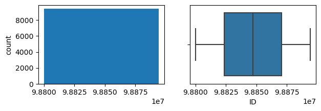
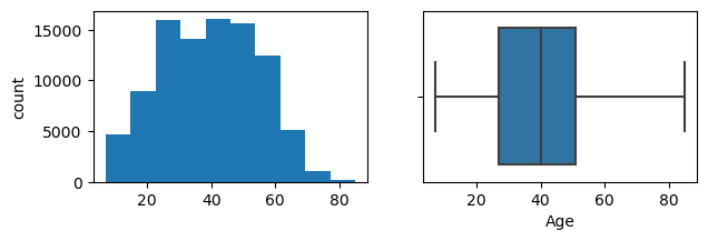
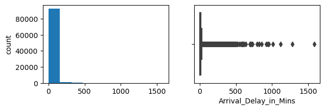
ID is not important, I will drop that. The median age of survey participants riding the bullet train is 40, and age looks almsot normally distributed. There is large range in the travel distance records. Departure and Arrival delays also look like they may be skewed. Lets plot these to get a better idea:
ID
Skew : 0.0
Age
Skew : -0.0
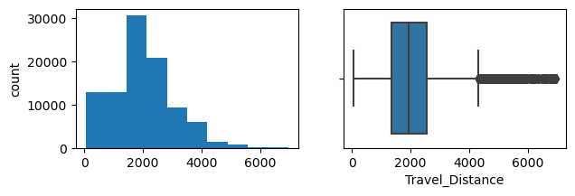
Travel_Distance
Skew : 0.47
Departure_Delay_in_Mins
Skew : 7.16

Arrival_Delay_in_Mins
Skew : 6.98
Overall_Experience
Skew : -0.19
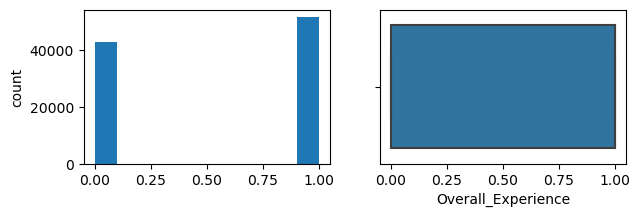
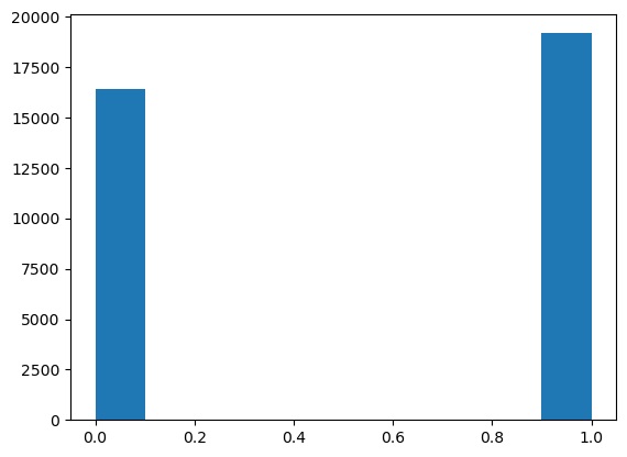
It looks like Age is actually more or less normally distributed. The more normal the features are, the better the classification models will perform (and the less I will need to transform). Travel Distance is somewhat right skewed, and as I suspected departure and arrival delays are highly right skewed. These will need to be dealt will. There are several different approaches one could take to normalize data like this in classification problems. The approach I take later in this analysis is to use feature engineering to bin the values into categories. Lets also take a look at the balance between negative and postiive overall experience:
1    0.546658
0    0.453342
Name: Overall_Experience, dtype: float64
There are marginally more positives than negatives, we can take balance into account when tuning the classifer models. Next, lets take a closer look at the categorical features:
Female    0.507041
Male      0.492959
Name: Gender, dtype: float64
****************************************
Loyal Customer       0.817332
Disloyal Customer    0.182668
Name: Customer_Type, dtype: float64
****************************************
Business Travel    0.688373
Personal Travel    0.311627
Name: Type_Travel, dtype: float64
****************************************
Eco         0.522807
Business    0.477193
Name: Travel_Class, dtype: float64
****************************************
Acceptable           0.224326
Needs Improvement    0.222079
Good                 0.218357
Poor                 0.160998
Excellent            0.137524
Extremely Poor       0.036716
Name: Seat_Comfort, dtype: float64
****************************************
Green Car    0.502601
Ordinary     0.497399
Name: Seat_Class, dtype: float64
****************************************
Good                 0.229072
Excellent            0.206954
Acceptable           0.177615
Needs Improvement    0.175426
Poor                 0.160236
Extremely Poor       0.050697
Name: Arrival_Time_Convenient, dtype: float64
****************************************
Acceptable           0.215652
Needs Improvement    0.209930
Good                 0.209825
Poor                 0.161821
Excellent            0.157115
Extremely Poor       0.045657
Name: Catering, dtype: float64
****************************************
Manageable           0.256208
Convenient           0.232244
Needs Improvement    0.189000
Inconvenient         0.174342
Very Convenient      0.148184
Very Inconvenient    0.000021
Name: Platform_Location, dtype: float64
****************************************
Good                 0.242027
Excellent            0.222239
Acceptable           0.213230
Needs Improvement    0.207697
Poor                 0.113843
Extremely Poor       0.000965
Name: Onboard_Wifi_Service, dtype: float64
****************************************
Good                 0.322654
Excellent            0.229374
Acceptable           0.186094
Needs Improvement    0.147582
Poor                 0.091574
Extremely Poor       0.022721
Name: Onboard_Entertainment, dtype: float64
****************************************
Good                 0.318344
Excellent            0.274627
Acceptable           0.166532
Needs Improvement    0.132657
Poor                 0.107829
Extremely Poor       0.000011
Name: Online_Support, dtype: float64
****************************************
Good                 0.306545
Excellent            0.262380
Acceptable           0.173796
Needs Improvement    0.153532
Poor                 0.103578
Extremely Poor       0.000170
Name: Ease_of_Online_Booking, dtype: float64
****************************************
Good                 0.314193
Excellent            0.245131
Acceptable           0.208244
Needs Improvement    0.131254
Poor                 0.101132
Extremely Poor       0.000046
Name: Onboard_Service, dtype: float64
****************************************
Good                 0.306186
Excellent            0.263361
Acceptable           0.173764
Needs Improvement    0.167071
Poor                 0.086012
Extremely Poor       0.003606
Name: Legroom, dtype: float64
****************************************
Good                 0.370810
Excellent            0.275932
Acceptable           0.188535
Needs Improvement    0.103558
Poor                 0.061165
Name: Baggage_Handling, dtype: float64
****************************************
Good                 0.281033
Acceptable           0.273621
Excellent            0.208278
Needs Improvement    0.118958
Poor                 0.118099
Extremely Poor       0.000011
Name: CheckIn_Service, dtype: float64
****************************************
Good                 0.375393
Excellent            0.276064
Acceptable           0.184894
Needs Improvement    0.103907
Poor                 0.059689
Extremely Poor       0.000053
Name: Cleanliness, dtype: float64
****************************************
Good                 0.270554
Acceptable           0.238151
Excellent            0.230384
Needs Improvement    0.142530
Poor                 0.118254
Extremely Poor       0.000127
Name: Online_Boarding, dtype: float64
****************************************
most of the categorical features are ordinal. This is important to note as we will need to encode them in preprocessing before running the models. There are no missing categories but there is imbalance in the percentage of data in each catagory (some categories are not very well represented). Finally, lets see if any of the features in the data are correlated:
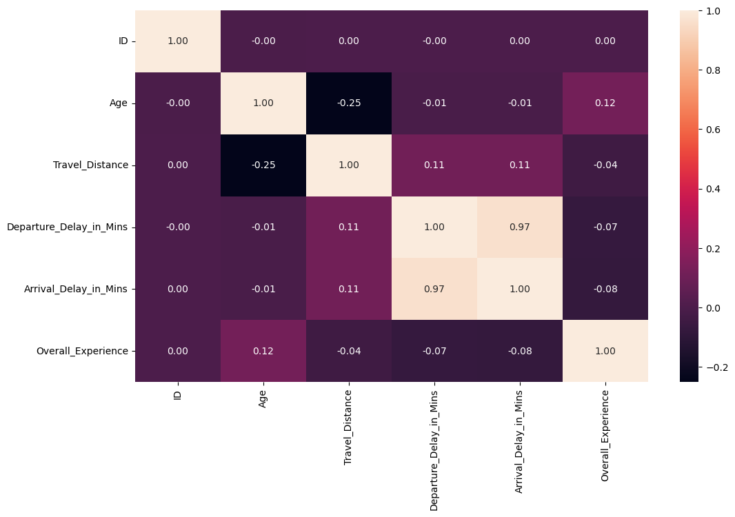
Arrival and Departure delay are highly correlated (suprise suprise :), but there is little correlation between any of the other numeric variables.
Preprocessing the training data
This is where Im going to drop the ID column out, and then split the data into the x (features) and y (target variable)
Im going to impute the numeric features using an iterative imputer to replace missing values based on all other features for a record, and categorical features will be replaced with the most frequent value for each column. After imputing, in the same code chunk, I encode the categorical features. Since most of the categorical features are oridinal, and there are many levels, I use the label_encoder method rather than one-hot encoding. With decision trees and random forest, one hot encoding can increase the number of features so much that it introduces ‘noise’ and leads to multicoliniarity.
Next, I bin the arrival and departure delay features to decrease the effect of skew and outliers
and make sure all of the features are numeric
Random Forest
RandomForestClassifier(random_state=7)In a Jupyter environment, please rerun this cell to show the HTML representation or trust the notebook.
On GitHub, the HTML representation is unable to render, please try loading this page with nbviewer.org.
RandomForestClassifier(random_state=7)
              precision    recall  f1-score   support

           0       1.00      1.00      1.00     42786
           1       1.00      1.00      1.00     51593

    accuracy                           1.00     94379
   macro avg       1.00      1.00      1.00     94379
weighted avg       1.00      1.00      1.00     94379

RandomForestClassifier(class_weight='balanced', max_depth=20, max_features=0.5,
                       n_estimators=150, random_state=7)
In a Jupyter environment, please rerun this cell to show the HTML representation or trust the notebook. On GitHub, the HTML representation is unable to render, please try loading this page with nbviewer.org.
RandomForestClassifier(class_weight='balanced', max_depth=20, max_features=0.5,
                       n_estimators=150, random_state=7)
precision recall f1-score support
0 0.99 1.00 1.00 42786
1 1.00 1.00 1.00 51593
accuracy 1.00 94379
macro avg 1.00 1.00 1.00 94379
weighted avg 1.00 1.00 1.00 94379
Now predicting y_test on x_test
XGBoost
XGBClassifier(base_score=0.5, booster='gbtree', callbacks=None,
              colsample_bylevel=1, colsample_bynode=1, colsample_bytree=1,
              early_stopping_rounds=None, enable_categorical=False,
              eval_metric='logloss', feature_types=None, gamma=0, gpu_id=-1,
              grow_policy='depthwise', importance_type=None,
              interaction_constraints='', learning_rate=0.300000012,
              max_bin=256, max_cat_threshold=64, max_cat_to_onehot=4,
              max_delta_step=0, max_depth=6, max_leaves=0, min_child_weight=1,
              missing=nan, monotone_constraints='()', n_estimators=100,
              n_jobs=0, num_parallel_tree=1, predictor='auto', random_state=1, ...)
In a Jupyter environment, please rerun this cell to show the HTML representation or trust the notebook. On GitHub, the HTML representation is unable to render, please try loading this page with nbviewer.org.
XGBClassifier(base_score=0.5, booster='gbtree', callbacks=None,
              colsample_bylevel=1, colsample_bynode=1, colsample_bytree=1,
              early_stopping_rounds=None, enable_categorical=False,
              eval_metric='logloss', feature_types=None, gamma=0, gpu_id=-1,
              grow_policy='depthwise', importance_type=None,
              interaction_constraints='', learning_rate=0.300000012,
              max_bin=256, max_cat_threshold=64, max_cat_to_onehot=4,
              max_delta_step=0, max_depth=6, max_leaves=0, min_child_weight=1,
              missing=nan, monotone_constraints='()', n_estimators=100,
              n_jobs=0, num_parallel_tree=1, predictor='auto', random_state=1, ...)
Now predicting y_test on x_test
| ID | Overall_Experience | |
|---|---|---|
| 0 | 99900001 | 1 |
| 1 | 99900002 | 1 |
| 2 | 99900003 | 1 |
| 3 | 99900004 | 0 |
| 4 | 99900005 | 1 |
this method had 0.9496 accuracy
XGBoost Regression
XGBRegressor(base_score=0.5, booster='gbtree', callbacks=None,
             colsample_bylevel=1, colsample_bynode=1, colsample_bytree=0.8,
             early_stopping_rounds=None, enable_categorical=False, eta=0.1,
             eval_metric=None, feature_types=None, gamma=0, gpu_id=-1,
             grow_policy='depthwise', importance_type=None,
             interaction_constraints='', learning_rate=0.100000001, max_bin=256,
             max_cat_threshold=64, max_cat_to_onehot=4, max_delta_step=0,
             max_depth=10, max_leaves=0, min_child_weight=0.5, missing=nan,
             monotone_constraints='()', n_estimators=1000, n_jobs=0,
             num_parallel_tree=1, predictor='auto', ...)
In a Jupyter environment, please rerun this cell to show the HTML representation or trust the notebook. On GitHub, the HTML representation is unable to render, please try loading this page with nbviewer.org.
XGBRegressor(base_score=0.5, booster='gbtree', callbacks=None,
             colsample_bylevel=1, colsample_bynode=1, colsample_bytree=0.8,
             early_stopping_rounds=None, enable_categorical=False, eta=0.1,
             eval_metric=None, feature_types=None, gamma=0, gpu_id=-1,
             grow_policy='depthwise', importance_type=None,
             interaction_constraints='', learning_rate=0.100000001, max_bin=256,
             max_cat_threshold=64, max_cat_to_onehot=4, max_delta_step=0,
             max_depth=10, max_leaves=0, min_child_weight=0.5, missing=nan,
             monotone_constraints='()', n_estimators=1000, n_jobs=0,
num_parallel_tree=1, predictor='auto', ...)| ID | Overall_Experience | |
|---|---|---|
| 0 | 99900001 | 1.0 |
| 1 | 99900002 | 1.0 |
| 2 | 99900003 | 1.0 |
| 3 | 99900004 | 0.0 |
| 4 | 99900005 | 1.0 |
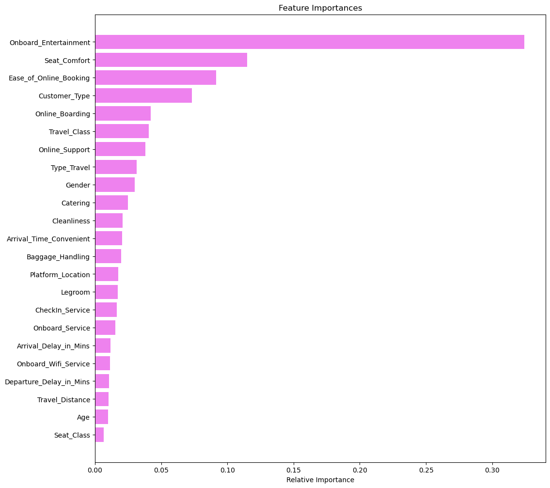
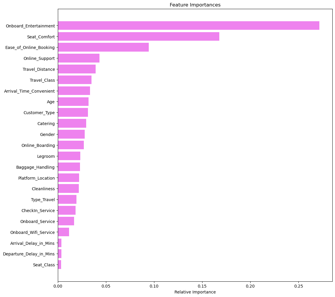
<AxesSubplot: >
Tuning hyperparameters of XGBoost Regression
Some important hyperparameters that can be tuned:
-
booster [default = gbtree ] Which booster to use. Can be gbtree, gblinear, or dart; gbtree and dart use tree-based models while gblinear uses linear functions.
-
min_child_weight [default = 1]
The minimum sum of instance weight (hessian) needed in a child. If the tree partition step results in a leaf node with the sum of instance weight less than min_child_weight, then the building process will give up further partitioning.The larger min_child_weight is, the more conservative the algorithm will be.
For a better understanding of each parameter in the XGBoost Classifier, please refer to this source.
Fitting 5 folds for each of 25 candidates, totalling 125 fits
XGBRegressor(base_score=0.5, booster='gbtree', callbacks=None,
             colsample_bylevel=0.5, colsample_bynode=1,
             colsample_bytree=0.8999999999999999, early_stopping_rounds=None,
             enable_categorical=False, eval_metric=None, feature_types=None,
             gamma=0, gpu_id=-1, grow_policy='depthwise', importance_type=None,
             interaction_constraints='', learning_rate=0.01, max_bin=256,
             max_cat_threshold=64, max_cat_to_onehot=4, max_delta_step=0,
             max_depth=20, max_leaves=0, min_child_weight=1, missing=nan,
             monotone_constraints='()', n_estimators=500, n_jobs=0,
             num_parallel_tree=1, predictor='auto', random_state=20, ...)
In a Jupyter environment, please rerun this cell to show the HTML representation or trust the notebook. On GitHub, the HTML representation is unable to render, please try loading this page with nbviewer.org.
XGBRegressor(base_score=0.5, booster='gbtree', callbacks=None,
             colsample_bylevel=0.5, colsample_bynode=1,
             colsample_bytree=0.8999999999999999, early_stopping_rounds=None,
             enable_categorical=False, eval_metric=None, feature_types=None,
             gamma=0, gpu_id=-1, grow_policy='depthwise', importance_type=None,
             interaction_constraints='', learning_rate=0.01, max_bin=256,
             max_cat_threshold=64, max_cat_to_onehot=4, max_delta_step=0,
             max_depth=20, max_leaves=0, min_child_weight=1, missing=nan,
             monotone_constraints='()', n_estimators=500, n_jobs=0,
             num_parallel_tree=1, predictor='auto', random_state=20, ...)
<AxesSubplot: >
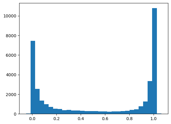
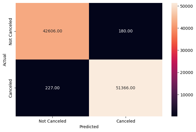
<AxesSubplot: >
This method had prediction accuracy of 0.9508455, placing 23 in the Great Learning Hack Linguist Hackathon Competition